|
Schur's
LRGB Color Correction Technique
A
schur fire method for true color LRGB astronomical images
By
Chris Schur and John Ofarrell
Uploaded 1/15/06
Note: I have intentionally
boosted the saturation of some of the images beyond normal amounts
to better demonstrate the concepts herein.
|
Abstract
Here we will
analyze the color distortion that occurs to the color image data
when we produce an LRGB image, and demonstrate a technique to
rebalance the LRGB back to the original precise G2V calibrated
RGB image.
Introduction
As astro-imagers,
we constantly push our cameras and gear to their limits to record
highly colorful and detailed images of faint deep sky objects.
There are two primary techniques used today for producing color
images but is missing the connection between them which must
exist to produce the most accurate and color correct photographs.
The first of these is what is called "G2V calibration".
While you can read about the details of doing such a calibration
here on
Al Kelly's web site, for this discussion we will first concern
ourselves with why we use this, and second, how to apply this
accurately produced color image to our second most popular technique
in the imagers toolbox: The LRGB color composite.
Why G2V Calibrate?
Anytime we produce
an image with a digital sensor, we take three images, each one
filtered with a different standardized color: Red, Blue and Green.
These images are then combined in software to produce the final
color image. But here's the catch - unless we standardize on
what we consider to be a white point, the three images can be
combined in any number of mixes and the colors will not be right.
Astrophotographers have chosen the color of our sun for the white
point, since it is central in our eyes color vision response,
and it appears as pure white to us in the daytime, when at the
zenith. (The sun is not yellow, take a sheet of white paper and
put it in the sun. What color is it?) Rather than go into a lengthy
discussion on why the G2V star such as our Sun was chosen as
white, I will say that each color gamut available such as Adobe
RGB, or LAB color space uses a different white point and we must
compensate. By using a standard candle so to speak for color,
we can now compare our images taken over large areas of the sky
and the spectrum of colors recorded by our cameras will look
similar in the final images. So my image of the Trifid nebula
will look just like yours, except for size. Direct comparison
with a common standard.
Why LRGB?
Soon after the
widespread use of color filters in CCD imaging was started back
in the 1980's, it became painfully apparent that long exposures
were needed through the dense color filters to get dim nebulosities
to show up. Producing a direct RGB image was not only extremely
time consuming, but also the long exposures made for tracking
errors, and focus shifts with amateur grade equipment. The solution
that emerged, and is now commonly used today for many deep and
detailed amateur shots is the technique of LRGB. Here we combine
a deep black and white full spectrum image with color frames
taken with the camera binned 2x2 or more to drastically shorten
the total exposure time for one subject. There are many sources
to read about producing LRGB images, for example one of the best
is Ron Wodaski's Advanced CCD imaging book. But there is a dilemma:
The LRGB image is convenient to make, but not color accurate.
So bad are the color distortions produced by introducing a new
Luminance image into the LAB color space or by combining with
layers as Luminosity in Photoshop, that they no longer resemble
the original calibrated G2V data we so painstakingly produced.
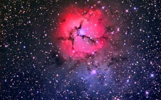
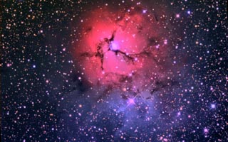
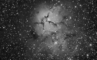
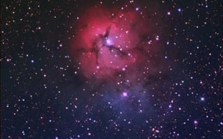
A typical LRGB
series
Below is an example
of a typical LRGB composite. On the left is a deep Luminance
image, that was binned at full resolution and has been processed
to bring out the maximum detail. In the middle is the G2V calibrated
color RGB frame, that was shot originally at 2x2 binning for
maximum color signal. Crisp reds and electric blues define the
beauty of this nebula clearly - but something happens to all
LRGB composites as illustrated on the right. The saturation is
obviously less, and the reds shift to the all to commonly seen
(this is all too common, unfortunately) salmon pink hue.
This is where most imagers stop, and consider the image done.
Obviously this does not resemble the right colors we started
with!
|
 Normal
Method of making LRGB image: L + RGB = LRGB ( --> Salmon Pink
!) Normal
Method of making LRGB image: L + RGB = LRGB ( --> Salmon Pink
!)
|
Understanding
and Rectifying the Problem
At the end of this
article John has put together the details of the mathematics
of producing the LRGB "Lab" composites and the color
shift issues. Here I will summarize the details of both the color
and saturation shift, and during our analysis a simple solution
will be presented.
Where the Color
Shift Comes From
When you combine
a Luminance frame into a color RGB data set, you will pass through
Lab color space. A direct method is to simply convert the RGB
data that has been scaled up in size to Lab color space, then
replace the "L" channel with a new highly detailed
deep frame. Alternately you can paste the new Luminance frame
right over the RGB data, and combine in layers with Luminance.
Or the third way is to paste the RGB image over the new Luminance
frame, and combine in layers using Color. They all come out the
same because Photoshop does the mathematics internally using
the Lab color space. In Lab mathematics, it can be shown that
the three channels are not completely separate. The "a"
channel is tied loosely with the L channel, but the "b"
channel is not significantly connected. The result is that if
you modify the L channel only, you will still change the "a
& b" channels proportionately. Now the "a"
channel controls the reds and oranges, and the "b"
channel the greens and blues. Since the "b" channel
is not significantly altered, it does not change hue as the brightness
of the L channel goes up. The "a" channel is a different
story! As you increase the brightness of the L channel, the "a"
channel shifts its hue. The result is that reds become more orange
resulting in the infamous "salmon pink" coloration,
while blues stay pretty much the same. This is what the math
predicts, and we will see in the examples below, that it bears
out well in an actual astronomical image.
Where the Color
Saturation is Lost.
Unlike the hue
shift which plagues only the "a" channel, as the Luminosity
in the "L" channel increases, both the "a"
and "b" channels will loose their saturation. Because
this is a non linear function, its is quite complex to predict
a correction factor. Just turning up the saturation in a standard
image processing software will only do a partial job. You can
visualize the loss in saturation as the whites start replacing
the colors at high brightness. The brighter the L channel gets
(or any RGB image), the greater the loss of color saturation
and contrasts. Many imagers try to compensate the salmon pink
shift in hue by simply turning up the saturation. You will see
below that this is quite unsatisfactory as well.
Demonstrating the
changes with CM
First I will introduce
you to a new imagers tool, created by professional photographers
to better understand and change the color tonalities in their
photographs. The version I am using comes standard with the full
Picture Window Pro software, but the Color Mechanic is available
separately as well for a lot less money. You can download a free
evaluation copy from www.dl-c.com and try it for yourself.
|
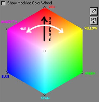 |
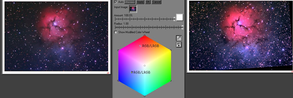
The
"Color Mechanic" Color Hexagon
On the left is
the color analysis and correction diagram of Digital Light and
Color's Color Mechanic. I have never found anything like it that
does color adjustments and changes such as this amazing tool.
Here's how it works, since you will need to understand it in
the next steps. The very center is pure white - the sum of all
colors equally. Three of the corners are the main RGB colors
we are familiar with in normal color work, and the other three
corners are exact even mixes of those three producing Cyan, Yellow
and Magenta. Full saturation is in the corners, and as you go
toward the center, the saturation decreases linearly. As you
move in a radius about the center white point, you shift the
Hue, or color frequency. When you click on a part of an image,
a small circle appears on the diagram corresponding to its hue
and saturation, allowing easy comparison of changes in our images.
Now that you have
a good feel for this tool, lets move on to analyze what happens
when you make an LRGB astronomical image.
|
|
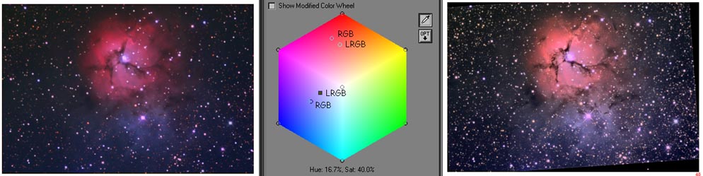
Both
a saturation and hue shift can be seen for the red and only a
saturation shift for the blue nebulosities.
By clicking on
the same exact spot on both images for both the red and blue
nebulosities, the true color shifts can be seen. In the red part
of the graphic at the top, the shift from RGB to LRGB is shifted
in both hue and saturation. You can see the LRGB is shifted more
into the oranges. If it had been saturation only, the shift would
be outward and inward toward the center. The blues on the other
hand are nearly unchanged in Hue, but affected about the same
as the reds in saturation. You can see if you were to move the
Blue RGB point directly inward toward the white center of the
hexagon, you would end up on the LRGB data. So as the math suggests,
reds are shifted both in hue and saturation, and blues and greens
will not change much in hue, yet be shifted in saturation as
well. So correction for the warm tones is a two step process:
First you correct the hue, then the saturation. You will still
want to do this to reflection nebulosities because often their
is a yellow or brown color to the dust, and of course the orange
stars will be corrected as well.
|
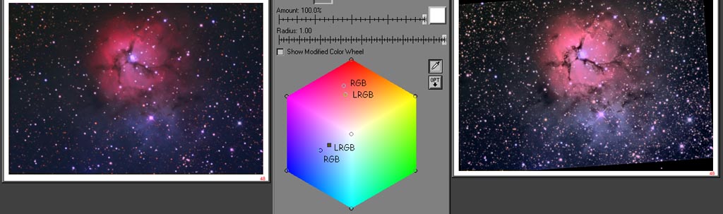
|
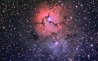
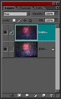
Hue
correction of LRGB on the left using layers in Photoshop and
combining with Hue, yields image on the right.
The first step
in correcting the LRGB image back to its G2V balanced origin,
is to correct the Hue. To do this is very easy. Layer your calibrated
RGB data (registered!) over the LRGB composite. Next as seen
in the center image above, select to combine the RGB image with
Hue at 100 percent transparency. The shift will be dramatic for
some images, less so for others. But in all cases - the new image
will have the correct hue of the original RGB. In fact, this
simple method you can do at any time during your normal color
processing to always bring it back to the standard color.
|
|
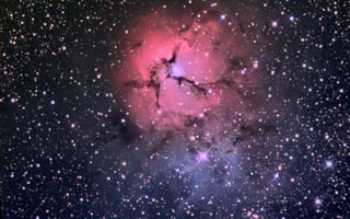
The
comparison shows the red has now been Hue shifted in frequency
to match RGB.
Now lets take a
look at what happed on the CM diagram. While the blues are about
the same, the reds took a dramatic turn and now line right up
with the central white zone. The beauty of this technique is
that ALL colors in the image will be corrected irrespective of
their end hue. Now you can see from the diagram, the only task
left is to correct the saturation.
|
|
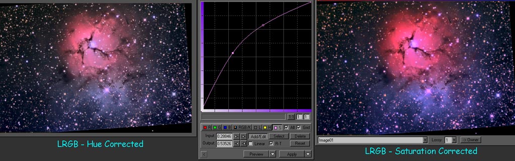
Next we implement the Hue Curves in PixInsight.
This is not your typical saturation boost! The curve boosts saturation
based on the existing amount of saturation, so areas with low
saturation such as dim nebulosity, and the bright core area will
be enhanced the most. Its really a wild concept. This takes care
of the change in saturation with increasing luminance which is
non linear.
Remember we discussed
how the saturation in an image is not linearly proportional to
the brightness increase of the L channel. Rather than a simple
brute force approach of cranking up the color saturation and
getting really poor results - which you will see demonstrated
below in a bit, we apply a special transfer function - a simple
gamma curve - to the saturation. Pix Insight is the only program
I've seen that allows this to be done this way. (And its freeware).
To under stand just what happened here, think of the plot above
as no saturation on the lower left, and increasing to maximum
saturation as you go right and up. You start with a straight
line from the lower left corner to the upper right which maps
1:1, just like a standard curves transfer function. Now when
we change this to a curve, the low saturations get boosted along
with the midranges. The top end doesn't change much. So we can
keep the saturation under control and give it where it needs
in - to the brightest areas that have lost the most. The dimmest
areas are also low in saturation and get a good boost too. You
can really see the blue come up wrapping around the red part
now.
|
 |
These two
images show the difference between a normal Photoshop saturation
boost, and the Pix saturation curves boost. |
 |
| The
left image is why you cant simply turn up the saturation normally.
Note the ring of intensely saturated reds around the edges of
nebula. They are maxed out and starting to red clip. But the
center of the nebula is still not nearly as a saturated red as
the original RGB data suggests. Thats the non linearity of this
creeping in. The right frame was corrected with the saturation
curve tool in PixInsight. No red fringe of over saturated color. |
|
The final
acid test - the original G2V calibrated RGB and the new LRGB
with correct color and much more structural detail.
You can see here
the pair of images now have overlapping samples when comparing
the original calibrated RGB image on the left to our finished
LRGB on the right. Both the reds and blues now line up perfectly.
The final LRGB now has stunning high resolution detail AND correct
colors. It is our hope that we can change your thinking on processing
LRGB images to a whole new level now. Don't drop the ball at
the finish line - go all the way and get that color right on
target !
|
LRGB Mathematics (John Ofarrell)
Many
amateur astrophotographers have experienced color shifts in red
nebula when using the LRGB method of enhancing their images.
An RGB image is made and converted into Lab color space. The
L channel is removed and replaced with enhanced data. The color
of the resulting image doesn't match the original RGB data.
Why is this? The answer lies in the details of the RGB to Lab
transformation. Since there are many flavors RGB color space,
we will use Adobe RGB (1998) color space for our discussion.
An RGB color space is defined in terms of red, green, and blue
color space primaries plus reference white and black points.
These five quantities are defined by X, Y, and Z coordinates
in CIE 1931 color space. The process for converting RGB to Lab
starts with aconversion of RGB to CIE 1931 XYZ. The XYZ color
coordinates are then converted to Lab. If one usesthe information
in "Adobe RGB (1998) Color Image Encoding" document
an expression for L in terms of RGB can be calculated. For the
remainder of this discussion we will assume that RGB is in the
form of 24-bit color with R, G, and B being represented by 8-bit
values. If we make a simplifying assumption that the reference
black point is X=Y=Z=0 then L as a function of RGB is as follows:
L = 116
[ 0.29734 R' + 0.62736 G' + 0.07529 B']^(1/3)- 16
where
R' = (R / 255)^(1/gamma), G' = (G/255) ^ (1/gamma), B' = (B/255)
^(1/gamma), and gamma= 2.19921875.
The value
of L can range between 1 and 100. Only for R=G=B=255 is L equal
to 100. So a saturated pixel in an L channel is white no matter
what was in the original RGB. Consider a pixel in an RGB image
that is pure red (R=255, G=0, and B=0), conversion to Lab gives
an L of 61. Thus any pure red pixel in the original RGB image
that has its L value replaced by a number greater than 61 has
to change color. So why doesn't the color just shift toward
the white? Why do
images end up with a "salmon pink" color? There is
no simple explanation. Salmon pink is essentially pink with
a little extra green added. Where does the extra green come
from? One can see from the equation for L as a function of R,
G, and B that L has the greatest
dependence on G. It seems reasonable that G will be most affected
by changes in L. All of this can be verified by setting up a
spread sheet that converts RGB to Lab and back again. The information
needed to convert Adobe RGB (1998) to XYZ can be found at Adobe's
website. The formulae for converting XYZ to Lab can be found
at www.brucelindbloom.com.
|
HOME SCHMIDT GALAXIES EMISSION NEBS REFLECTION NEBS COMETS
GLOBULARS OPEN CLUST PLANETARIES LINKS
|
|
 Look VERY carefully, its pinker.