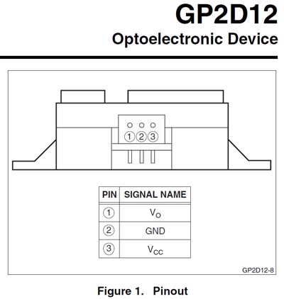

Overview:
This sensor belongs to a family of optical distance sensors made by Sharp and several other manufacturers. It function is somewhere in between a acoustical sonar and a Lidar laser range finder. This sharp device projects a modulated IR beam onto a target, and senses the centroid of the received image with a camera type sensor and the output is an analog voltage that is inversely proportional to the distance. The useful range is from 9cm to 80cm (3 - 30") and is accurate when properly calibrated to better than half an inch.
The sensor is in a black plastic housing, and is roughly an inch in size. Two black lenses that are dyed with an infrared pass filter are on the front. Internally, the source of the beam is an IR LED which projects a roughly circular beam about 1/4 inch in diameter out. It expands slowly to one inch at the maximum distance of 80cm.
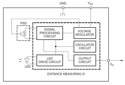
Internally, the sensor is quite complex. It contains a small processor and drive circuitry for operation. the PSD sensor is the key - it is a silicon sensor called a Position Sensing Device. These are basically a silicon die with leads bonded on both sides like a solar cell. But they read out differentially relative to the ground plane and the closer a bright spot is to the lead, the larger the signal. This creates a +/- offset which is amplified and fed to the processor.
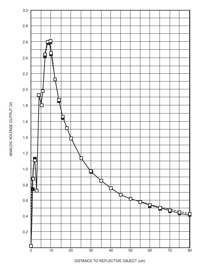
This is the transfer function that Sharp provides for the response at various distances. You can see that between 0 and 9cm the sensor is too close for the optical triangulation to work, and the true curve starts after that. It decays exponentially in a 1/x manner.
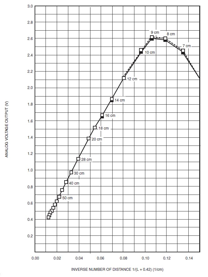
Sharp also provides this enlightening graph. It shows the X axis as a number as N = 1/(L + .42) which is a clue to linearization of the data. The line does deviate slightly from flat due to non linearities in the sensor and optics.
Linearization Math
From the manufacturers second nearly straight line graph, we can first extract the slope m from rise/run = m. Using the full length of data, I get m = 2.2/.094 = 23.4 , and extending the line downward, the y intercept (b) is exactly .1
Using the standard straight line formula y = mx + b, we derive x = (y-b)/m. So when we measure the voltage output, we substitute these known values in the equation to derive N. So for example:
for 2.6v for the 9cm distance, N = (2.6 - .1)/23.4 = .106
This derives the value for the x axis value N. From the equation they provide along the X axis then of N = 1/(L + .42) we can solve for L as L = (1/N) - .42 where L is the distance in centimeters. Plugging in the number of N from our 2.6v measurement we get L = (1/.106) - .42
which equals L = 9cm. Convert to inches by dividing by 2.54 and L = 3.5".
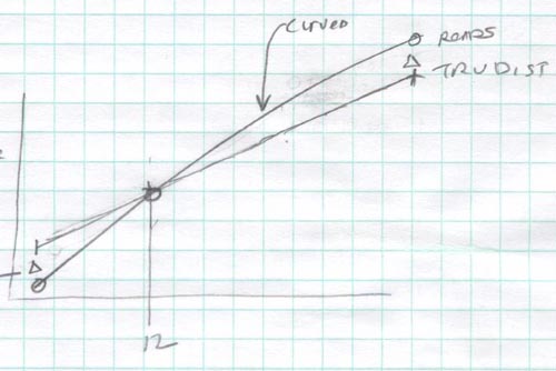
Finally, the resulting curve is nearly straight but slightly concave downward from non linearities in the device and optics. A final calibration correction was applied to the data using the standard cal formula New dist = (multiplier * inches) + Additive shift. The correction to the initial calculated distance in inches was then D = (.9 * d) + 1.2 this corrected the curve such that the errors on the ends were the same as the 12 inch point which was the intersection and thus the correct reading. As you get closer to the sensor, it read higher and farther than 12 inches it read lower as seen in the graph below. Final accuracy was within a half inch over the entire range.
The upper curve then which is concave downward must be adjusted mathematically to show equal error on both ends and the middle points for best accuracy. Note at 12 inches, the two graphs cross and thus is accurate. The goal is to change the curve to most closely match the linear line. This equation set was programmed into the PIC after the raw voltage was measured on the sensor with the analog 0 input. Of course the analog value is digitized to 12 bit resolution, and this would be converted to actual voltage because we know the mv/bit = 4.88
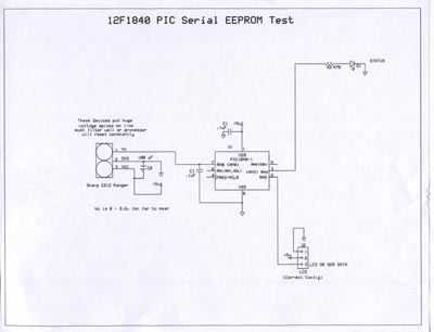
Schematic for my test circuit. A 12F1840 PIC processor is used to sample the analog output and perform the calculations. The resulting distance in inches is displayed on the LCD. Note the large capacitor on the sensor. This is required because of the huge current spikes that the sensor puts on the power line! Without this, the spikes will constantly reset the processor.
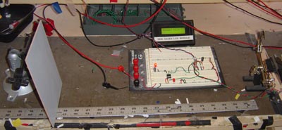
Bench Setup. The target is on the left and we can vary the distance from the sensor, which is in a black housing on the right held by a clamp. The LCD is above center and reads out rapidly the distance to two decimal places.
Conclusion:
Approximately half inch resolution was achieved over the full 30 inch range with this setup. This is sufficient for robot navigation in smaller areas and maneuvering around obstacles. It also allows 3D mapping of the area around the robot and thus some object identification is possible.
Code for the 12f1840 PIC:
//****************************************************************************
//Chris Schur
//(Program Name): 12F1840 Tests with Sharp GD12 Ranger
//Date: 2/16/18
//****************************************************************************/*Description.
v6 added cal factor to get close as possible with actual. The final line is
still curved downward a bit, so cal attempts to equalize the errors over
the whole range.V7 FUNCTIONALIZED.works great.*/
//I/O Designations ---------------------------------------------------
// A0 (RA0): Vin Ranger
// A1 (RA1): x
// A2 (RA2): x
// A3 (RA3): x (can ONLY be input)
// A4 (RA4): Status LED
// A5 (RA5): LCD
//--------------------------------------------------------------------
//Include Files:
#include <12F1840.h> //Normally chip, math, etc. used is here.#device ADC=10
//Directives and Defines:
#fuses NOPROTECT,NOMCLR
#use delay(internal=4000000)
#use fast_io(A)//for new New Haven 16 x 2 Serial LCD:
#use rs232(baud=9600, xmit=Pin_A5, bits=8, parity=N, stream=SERIALNH)
//****************************************************************************
//Global Variables:
//****************************************************************************
int16 RESULT; //a/d conversion of sensor
float VOUT; //voltage conversion from raw
float L; //distance in cm
float NN; //N number for calculations
float IN; //distance in inches
//Functions/Subroutines, Prototypes:
void LCDCLR(); //Clears LCD Display:
void LCDLN2(); //Sets LCD to line 2 start point
void READSHARP(); //Reads Sharp sensor, returns dist.//****************************************************************************
//-- Main Program
//****************************************************************************void main(void) {
// Set TRIS I/O directions, define analog inputs, compartors:
//(analog inputs digital by default)
set_tris_A(0b001111);
setup_adc_ports(sAN0); //sensor v input is 0 - 5v
setup_adc(ADC_CLOCK_DIV_32);
set_adc_channel(0);//Initialize variables and Outputs: --------------------------------------
RESULT = 0;
delay_ms(1000); //lcd warmup
//----------------------------------------------------------------
LCDCLR(); //initial splash screen
delay_ms(25);
fprintf(SERIALNH,"SHARP1");
delay_ms(1000); //Display time
//MAIN LOOP:
while(true) {output_high(PIN_A4);
delay_ms(10);READSHARP();
LCDCLR(); //read out data
delay_ms(25);
fprintf(SERIALNH,"Inches= %f",IN);
delay_ms(25); //Display time
output_low(PIN_A4);
delay_ms(50);}
}
//********* Functions which have prototypes at top of program ****************
//functions for NEW HAVEN LCD display:
//Clears LCD Display:
void LCDCLR() {
fputc(0xFE,SERIALNH); //Command Prefix
fputc(0x51,SERIALNH); //Clear screen
}//Sets LCD to line 2 start point
void LCDLN2() {
fputc(0xFE,SERIALNH); //Command Prefix
fputc(0x45,SERIALNH); //set cursor command
fputc(0x40,SERIALNH); //Set cursor to next line, pos 40 = start line 2
}void READSHARP() { //Reads Sharp sensor, returns dist.
//take reading on analog 0 input:
RESULT = read_adc(); //12 BIT DATA
//next we calculate voltage:
//4.883 mv/bit for 10 bit a/d
VOUT = RESULT * .004883;//Next we limint Vo so that it not exceed low limit (gets neg numbers for NN)
if(VOUT < .4)
VOUT = .4;//next we calculate from voltage N number. the formula is:
// we know y = mx + b, solving for x, x = y-b/m. From thier graph, the slope is
//m = rise/run = 2.2/.094 = 23.40. and the Y intercept (b) is .1
// N = (y-b)/m:
NN = (VOUT - .1)/23.4;//Next L which is dist in cm:
//L = (1/N)-.42:
L = (1/NN) - .42;//Next calculate distance in inches:
IN = L/2.54;//Final cal to match actual measures. inches = (inches * K) + offset.
IN = (IN * .9) + 1.2;}